Visualize Parsed GenDC Data

In this tutorial, we learn how to visualize sample GenDC Data parsed in the previous tutorial.

Prerequisite

• GenDC Separator
• matplotlib
• numpy

pip3 install -U pip
pip3 install matplotlib
pip3 install numpy
pip3 install gendc-python==0.2.8

• GenDC Data (obtained in the previous tutorial or Download sample from this page).

Tutorial

In the previous tutorial, we learned how to parse GenDC data from a binary file. After obtain each Part data, we can reshape it to use in your application. In this tutorial, we can

note

We will use sample data in this tutorial.

GenDC

If you would like to learn the overview of GenDC, please check this page that gives you the concept and rough structure of GenDC.

Find and load Binary file

Check the previous tutorial to load binary file. At the Part, you can obtain raw-data of image.

binary_image = part.get_data()

Visualize Image

In the previous tutorial, we obtained that the Component having image data, which is 0.

Also, we have the following data:

• dimension = (1920, 1080)
• byte_depth = 1

With these properties, we can put binary-image data into numpy array of uint8.

np_image = np.frombuffer(binary_image, dtype=get_numpy_dtype(byte_depth, unsinged=True))

Since the current np_image is just a 1D array, we can reshape it into width x height shape.

Note that dimension obtained by get_dimension() returns in the order of width by height of the image, while matplotlib requires the dimension in the order of height then width.

WxH = dimension
HxW = dimension[::-1]
image_data = np_image.reshape(HxW)

The code snippets above can be written in the single line as follws:

image_data = np.frombuffer(part.get_data(), dtype=get_numpy_dtype(byte_depth, unsinged=True)).reshape(dimension[::-1])

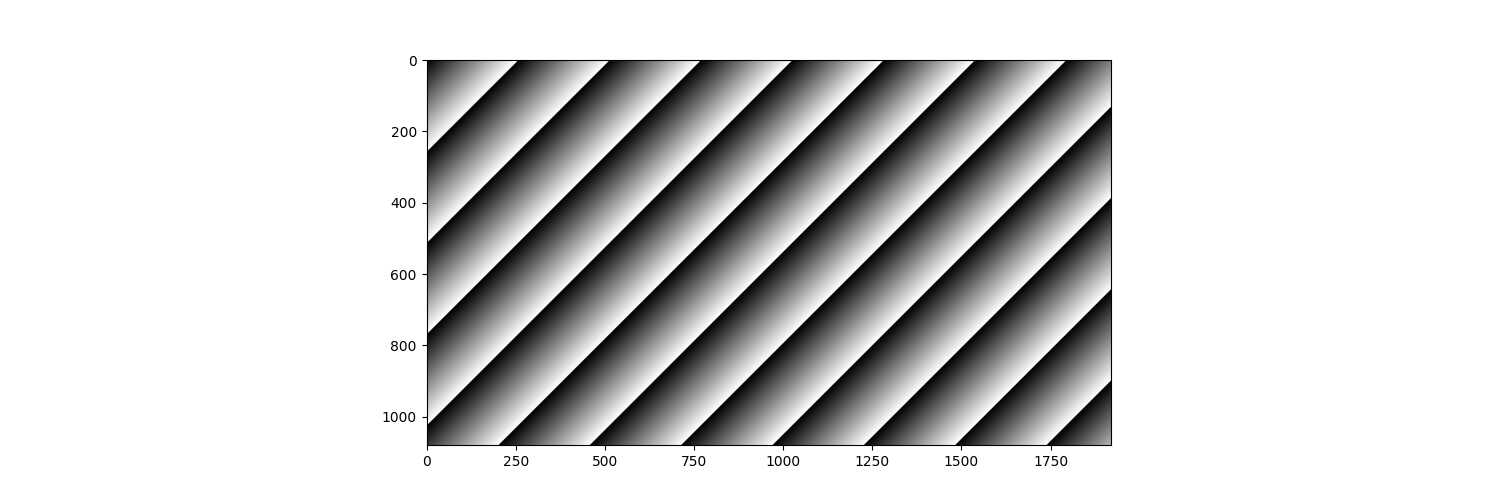
Now, we can display image data with imshow().

image_fig = plt.figure(figsize=(15, 5))
plt.imshow(image_data, cmap='gist_gray')
plt.show()

.

Visualize Audio Data

In the previous tutorial, we obtained that the Component having audio data, which is 1.

Also, we have the following data:

• channel = 2
• dimension = (800,)
• byte_depth = 2

With these properties, we can put binary-image data into numpy array of int16 as we did for image Component.

for j in range(part_count):
    part = audio_component.get_part_by_index(j)
    dimension = (800,)
    byte_depth = 2

    audio_part_data = np.frombuffer(part.get_data(), dtype=get_numpy_dtype(byte_depth, unsinged=False)).reshape(dimension)

This audio sensor data store samples obtained during the time it takes to acquire one frame of that image data, which is 60fps.

Therefore, time duration is 0 to 1/60 s.

num_samples = audio_part_data.shape[0]
times = np.linspace(0, 1/image_fps, num=num_samples)[:num_samples]

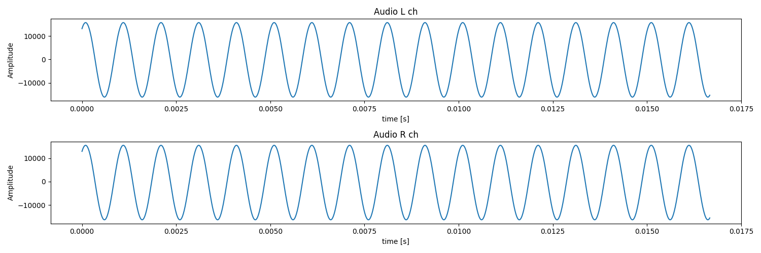
We can put 2 Part diagams in the same figure by using subplot as follows:

audio_fig = plt.figure(figsize=(15, 5))
for j in range(part_count):
    part = audio_component.get_part_by_index(j)
    dimension = (800,)
    byte_depth = 2

    audio_part_data = np.frombuffer(part.get_data(), dtype=get_numpy_dtype(byte_depth, unsinged=False)).reshape(dimension)

    ax = audio_fig.add_subplot(part_count, 1, j+1)
    ax.plot(times, audio_part_data)
plt.show()

.

info

Some of audio sensor uses interleaved audio, which store Lch and Rch in the same Part in turns. In this case, audio_component.get_part_count() returns 1, but you need to re-shape the data into 2-dim to use it as follows:

part = audio_component.get_part_by_index(j)
dimension = (800, 2)
byte_depth = 2

audio_part_data = np.frombuffer(part.get_data(), dtype=get_numpy_dtype(byte_depth, unsinged=False)).reshape(dimension)

Lch_data = audio_part_data[:, 0]
Rch_data = audio_part_data[:, 1]

Visualize Analog Data

In the previous tutorial, we obtained that the Component having audio data, which is 2, 3, and 4.

Also, we have the following data:

• channel = 1
• dimension = (16,)
• byte_depth = 2

We can obtain Part data and generate time line for X-axis as we learned:

for j in range(part_count):
    part = analog_component.get_part_by_index(j)
    dimension = (16,)
    byte_depth = 2

    analog_part_data = np.frombuffer(part.get_data(), dtype=get_numpy_dtype(byte_depth, unsinged=False)).reshape(dimension)
    num_samples = analog_part_data.shape[0]

    times = np.linspace(0, num_samples/(image_fps * num_samples), num=num_samples)[:num_samples]

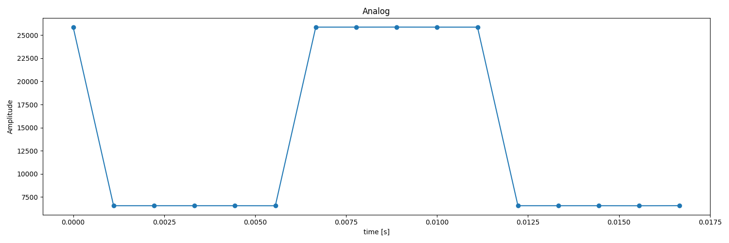
Dimension represents the number of samples obtain in 1/60 s, so you may see 16 dots in the visualization:

analog_fig = plt.figure(figsize=(15, 5))
ax = analog_fig.add_subplot(1, 1, +1)
ax.plot(times, analog_part_data, marker = 'o')
plt.show()

.

Visualize PMOD Data

In the previous tutorial, we obtained that the Component having accelerometer data, which is 5.

Also, we have the following data:

• channel = 3
• dimension = (16,)
• byte_depth = 2

Each Part represents the coordinate of X, Y, and Z, so we append each Part data into the list of XYZ.

XYZ = []

for j in range(part_count):
    part = pmog_component.get_part_by_index(j)
    dimension = (16,)
    byte_depth = 2

    pmod_part_data = np.frombuffer(part.get_data(), dtype=get_numpy_dtype(byte_depth, unsinged=False)).reshape(dimension)
    XYZ.append(pmod_part_data)

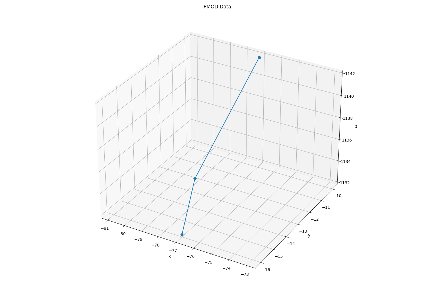
Now, we can plot XYZ to 3D space to see the acceleration of the camera. Since the sensor was not accelerating at some point, the number of the samples may look less than 16.

pmod_fig = plt.figure(figsize=(15, 10))
ax = pmod_fig.add_subplot(projection='3d')
ax.plot(XYZ[0], XYZ[1], XYZ[2], marker = 'o')
plt.show()

.

info

Some of accelerometer sensor uses interleaved structure, which store X, Y, and Z coordinate in the same Part in turns. In this case, pmog_component.get_part_count() returns 1, but you may need to re-shape the data into 4-dim (x, y, z, and padding) to use it as follows:

part = pmod_component.get_part_by_index(j)
dimension = (800, 4)
byte_depth = 2

pmod_part_data = np.frombuffer(part.get_data(), dtype=get_numpy_dtype(byte_depth, unsinged=False)).reshape(dimension)

X = pmod_part_data[:, 0]
Y = pmod_part_data[:, 1]
Z = pmod_part_data[:, 2]

Complete code

Complete code used in the tutorial is here.